Tensorflow 2.0實現Fashion MNIST實驗

　　本指南使用的是tf.keras，它是一種用于在 TensorFlow 中構建和訓練模型的高階 API。

1.導入相關庫

from __future__ import absolute_import, division, print_function, unicode_literals

# TensorFlow and tf.keras
import tensorflow as tf
try:
    import tensorflow.keras as keras
except:
    import tensorflow.python.keras as keras
# Helper libraries
import numpy as np
import matplotlib.pyplot as plt
print(tf.__version__)

2.導入MNIST數據集

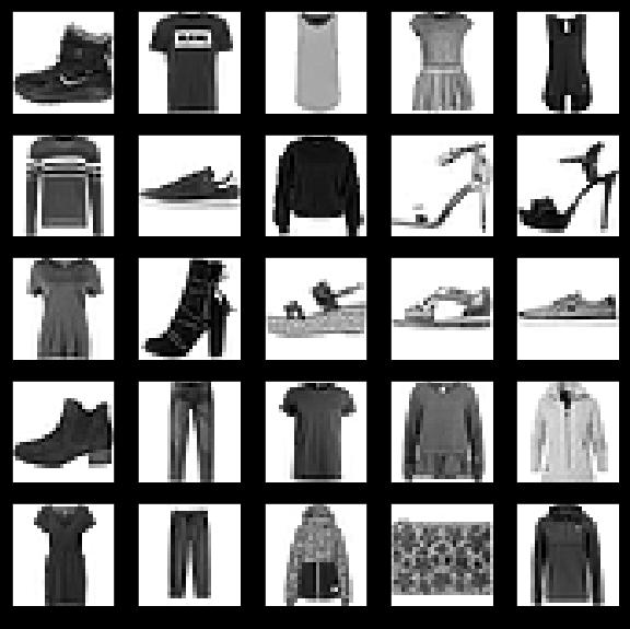
　　本指南使用Fashion MNIST <https://github.com/zalandoresearch/fashion-mnist>數據集，其中包含 70000 張灰度圖像，涵蓋 10 個類別。以下圖像顯示了單件服飾在較低分辨率（28x28 像素）下的效果：

Fashion MNIST sprite

    train_images和train_labels數組是訓練集，即模型用于學習的數據。
    測試集 test_images 和 test_labels 數組用于測試模型。
圖像為28x28的NumPy數組，像素值介于0到255之間。標簽是整數數組，介于0到9之間。這些標簽對應于圖像代表的服飾所屬的類別：

class_names = ['T-shirt/top', 'Trouser', 'Pullover', 'Dress', 'Coat',
               'Sandal', 'Shirt', 'Sneaker', 'Bag', 'Ankle boot']

3.探索數據

我們先探索數據集的格式，然后再訓練模型。以下內容顯示訓練集中有 60000 張圖像，每張圖像都表示為 28x28 像素：

train_images.shape
 (60000, 28, 28)
同樣，訓練集中有60,000個標簽：
len(train_labels)
60000
每個標簽都是0到9之間的整數：
train_labels
array([9, 0, 0, ..., 3, 0, 5], dtype=uint8)
測試集中有10,000個圖像。同樣，每個圖像表示為28 x 28像素：
test_images.shape
 (10000, 28, 28)
測試集包含10,000個圖像標簽：
len(test_labels)
10000

4.預處理數據

在訓練網絡之前必須對數據進行預處理。 如果您檢查訓練集中的第一個圖像，您將看到像素值落在0到255的范圍內：

#預處理數據
plt.figure()
plt.imshow(train_images[0])
plt.colorbar()
plt.grid(False)
plt.show()
我們將這些值縮小到 0 到 1 之間，然后將其饋送到神經網絡模型。為此，將圖像組件的數據類型從整數轉換為浮點數，然后除以 255。以下是預處理圖像的函數：務必要以相同的方式對訓練集和測試集進行預處理：
train_images = train_images / 255.0
test_images = test_images / 255.0
為了驗證數據的格式是否正確以及我們是否已準備好構建和訓練網絡，讓我們顯示訓練集中的前25個圖像，并在每個圖像下方顯示類名。
plt.figure(figsize=(10,10))
for i in range(25):
    plt.subplot(5,5,i+1)
    plt.xticks([])
    plt.yticks([])
    plt.grid(False)
    plt.imshow(train_images[i], cmap=plt.cm.binary)
    plt.xlabel(class_names[train_labels[i]])
plt.show()

5.構建模型

模型還需要再進行幾項設置才可以開始訓練。這些設置會添加到模型的編譯步驟：
    損失函數：衡量模型在訓練期間的準確率。我們希望盡可能縮小該函數，以“引導”模型朝著正確的方向優化。
    優化器：根據模型看到的數據及其損失函數更新模型的方式。
    度量標準：用于監控訓練和測試步驟。以下示例使用準確率，即圖像被正確分類的比例。
model.compile(optimizer='adam',
              loss='sparse_categorical_crossentropy',
              metrics=['accuracy'])

6.訓練模型

model.fit(train_images, train_labels, epochs=5)

7.評估精度

接下來，比較模型在測試數據集上的表現情況：

test_loss, test_acc = model.evaluate(test_images, test_labels)
print('\nTest accuracy:', test_acc)
輸出：
10000/10000 [==============================] - 1s 50us/step
Test accuracy: 0.8734
結果表明，模型在測試數據集上的準確率略低于在訓練數據集上的準確率。訓練準確率和測試準確率之間的這種差異表示出現過擬合(overfitting)。如果機器學習模型在新數據上的表現不如在訓練數據上的表現，也就是泛化性不好，就表示出現過擬合。

8.預測

???輸出：
array([6.2482708e-05, 2.4860196e-08, 9.7165821e-07, 4.7436039e-08,
       2.0804382e-06, 1.3316551e-02, 9.8731316e-06, 3.4591161e-02,
       1.2390658e-04, 9.5189297e-01], dtype=float32)
?預測結果是一個具有 10 個數字的數組，這些數字說明模型對于圖像對應于 10 種不同服飾中每一個服飾的“confidence（置信度）”。我們可以看到哪個標簽的置信度值較大：
np.argmax(predictions[0])

因此，模型非常確信這張圖像是踝靴或屬于 class_names[9]。我們可以檢查測試標簽以查看該預測是否正確：
test_labels[0]
我們可以將該預測繪制成圖來查看全部 10 個通道
def plot_image(i, predictions_array, true_label, img):
  predictions_array, true_label, img = predictions_array[i], true_label[i], img[i]
  plt.grid(False)
  plt.xticks([])
  plt.yticks([])

  plt.imshow(img, cmap=plt.cm.binary)

  predicted_label = np.argmax(predictions_array)
  if predicted_label == true_label:
    color = 'blue'
  else:
    color = 'red'

  plt.xlabel("{} {:2.0f}% ({})".format(class_names[predicted_label],
                                100*np.max(predictions_array),
                                class_names[true_label]),
                                color=color)

def plot_value_array(i, predictions_array, true_label):
  predictions_array, true_label = predictions_array[i], true_label[i]
  plt.grid(False)
  plt.xticks([])
  plt.yticks([])
  thisplot = plt.bar(range(10), predictions_array, color="#777777")
  plt.ylim([0, 1])
  predicted_label = np.argmax(predictions_array)

  thisplot[predicted_label].set_color('red')
  thisplot[true_label].set_color('blue')

讓我們看看第0個圖像，預測和預測數組。??

i = 0
plt.figure(figsize=(6,3))
plt.subplot(1,2,1)
plot_image(i, predictions, test_labels, test_images)
plt.subplot(1,2,2)
plot_value_array(i, predictions,  test_labels)
plt.show()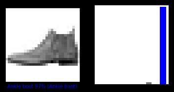
?

i = 12
plt.figure(figsize=(6,3))
plt.subplot(1,2,1)
plot_image(i, predictions, test_labels, test_images)
plt.subplot(1,2,2)
plot_value_array(i, predictions,  test_labels)
plt.show()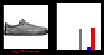
?

我們用它們的預測繪制幾張圖像。正確的預測標簽為藍色，錯誤的預測標簽為紅色。數字表示預測標簽的百分比（總計為 100）。請注意，即使置信度非常高，也有可能預測錯誤。
# 繪制前X個測試圖像，預測標簽和真實標簽。 
# 用藍色標記正確的預測，用紅色標記錯誤的預測。
num_rows = 5
num_cols = 3
num_images = num_rows*num_cols
plt.figure(figsize=(2*2*num_cols, 2*num_rows))
for i in range(num_images):
  plt.subplot(num_rows, 2*num_cols, 2*i+1)
  plot_image(i, predictions, test_labels, test_images)
  plt.subplot(num_rows, 2*num_cols, 2*i+2)
  plot_value_array(i, predictions, test_labels)
plt.show()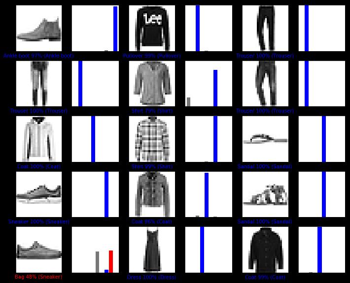
??

最后，使用訓練的模型對單個圖像進行預測。
# 從測試數據集中獲取圖像
img = test_images[0]

print(img.shape)
tf.keras模型已經過優化，可以一次性對樣本批次或樣本集進行預測。因此，即使我們使用單個圖像，仍需要將其添加到列表中：
# 將圖像添加到批次中，它是唯一的成員。
img = (np.expand_dims(img,0))

print(img.shape)
 (1, 28, 28)
現在預測此圖像的正確標簽：
predictions_single = model.predict(img)
print(predictions_single)
plot_value_array(0, predictions_single, test_labels)
_ = plt.xticks(range(10), class_names, rotation=45)
?

model.predict返回一組列表，每個列表對應批次數據中的每張圖像。（僅）獲取批次數據中相應圖像的預測結果：
np.argmax(predictions_single[0])

本實驗利用網上已有的北京房價數據集預測了北京的房價，實現了TensorFlow的線性回歸應用。?